Error Detection and Correction

 Error Detection and Correction

Data can be corrupted during transmission. Some applications require that errors be detected and corrected. 

Types of Errors

Single-Bit Error

Burst Error

Single-Bit Error

In a single-bit error, only 1 bit in the data unit has changed.

Burst Error

A burst error means that 2 or more bits in the data unit have changed.

Redundancy-

The central concept in detecting or correcting errors is redundancy. To be able to detect or correct errors, we need to send some extra bits with our data. These redundant bits are added by the sender and removed by the receiver. Their presence allows the receiver to detect or correct corrupted bits.

Detection Versus Correction
The correction of errors is more difficult than the detection. In error detection, we are looking only to see if any error has occurred. The answer is a simple yes or no. We are not even interested in the number of errors. A single-bit error is the same for us as a burst error.

In error correction, we need to know the exact number of bits that are corrupted and more importantly, their location in the message. The number of the errors and the size of the message are important factors. If we need to correct one single error in an 8-bit data unit, we need to consider eight possible error locations; if we need to correct two errors in a data unit of the same size, we need to consider 28 possibilities. You can imagine the receiver's difficulty in finding 10 errors in a data unit of 1000 bits

Vertical Redundancy Check (VRC) or Parity Check-

Vertical Redundancy Check is also known as Parity Check. In this method, a redundant bit also called parity bit is added to each data unit. This method includes even parity and odd parity. Even parity means the total number of 1s in data is to be even and odd parity means the total number of 1s in data is to be odd. Example - If the source wants to transmit data unit 1100111 using even parity to the destination. The source will have to pass through Even Parity Generator. 

 

Advantages :

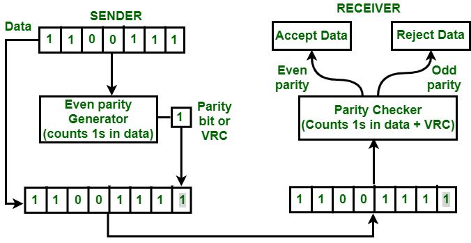
• VRC can detect all single bit error.
• It can also detect burst errors but only in those cases where number of bits changed is odd, i.e. 1, 3, 5, 7, .......etc.
• VRC is simple to implement and can be easily incorporated into different communication protocols and systems.
• It is efficient in terms of computational complexity and memory requirements.
• VRC can help improve the reliability of data transmission and reduce the likelihood of data corruption or loss due to errors.
• VRC can be combined with other error detection and correction techniques to improve the overall error handling capabilities of a system.

Disadvantages : 

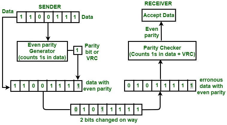
• The major disadvantage of using this method for error detection is that it is not able to detect burst error if the number of bits changed is even, i.e. 2, 4, 6, 8, .......etc. 
• Example - If the original data is 1100111. After adding VRC, data unit that will be transmitted is 11001111. Suppose on the way 2 bits are 01011111. When this data will reach the destination, parity checker will count number of 1s in data and that comes out to be even i.e. 8. So, in this case, parity is not changed, it is still even. Destination will assume that there is no error in data even though data is erroneous.
• VRC is not capable of correcting errors, only detecting them. This means that it can identify errors, but it cannot fix them.
• VRC is not suitable for applications that require high levels of error detection and correction, such as mission-critical systems or safety-critical applications.
• VRC is limited in its ability to detect and correct errors in large blocks of data, as the probability of errors increases with the size of the data block.
• VRC requires additional overhead bits to be added to the data stream, which can increase the bandwidth and storage requirements of the system.

 

 

Longitudinal Redundancy Check (LRC) is also known as 2-D parity check. In this method, data which the user want to send is organized into tables of rows and columns. A block of bit is divided into table or matrix of rows and columns. In order to detect an error, a redundant bit is added to the whole block and this block is transmitted to receiver. The receiver uses this redundant row to detect error. After checking the data for errors, receiver accepts the data and discards the redundant row of bits. Example : If a block of 32 bits is to be transmitted, it is divided into matrix of four rows and eight columns which as shown in the following figure : 

 

 

 

In this matrix of bits, a parity bit (odd or even) is calculated for each column. It means 32 bits data plus 8 redundant bits are transmitted to receiver. Whenever data reaches at the destination, receiver uses LRC to detect error in data. Advantage : LRC is used to detect burst errors. Example : Suppose 32 bit data plus LRC that was being transmitted is hit by a burst error of length 5 and some bits are corrupted as shown in the following figure :  

 

The LRC received by the destination does not match with newly corrupted LRC. The destination comes to know that the data is erroneous, so it discards the data. Disadvantage : The main problem with LRC is that, it is not able to detect error if two bits in a data unit are damaged and two bits in exactly the same position in other data unit are also damaged. Example : If data 110011 010101 is changed to 010010110100.  

 

 

 Checksum 

• In checksum error detection scheme, the data is divided into k segments each of m bits.
• In the sender’s end the segments are added using 1’s complement arithmetic to get the sum. The sum is complemented to get the checksum.
• The checksum segment is sent along with the data segments.
• At the receiver’s end, all received segments are added using 1’s complement arithmetic to get the sum. The sum is complemented.
• If the result is zero, the received data is accepted; otherwise discarded.